Examples
modified 18 March 2024 by Paweł Netzel
In following examples, you can find hints and different approaches to using plMapcalc. Examples are ordered from simplest to the most complex. All examples are dedicated to run in Linux. Windows system needs small modifications: different path element separator (in options -i,-o,-r,-s) and double quotation marks (in option -e).
- Example 1: adding two (or more) layers
- Example 2: calculation of NDVI
- Example 3: a mask file creating
- Example 4: statistics calculation
- Example 5: reclassification of input layer
- Example 6: area calculation and assigning
- Example 7: space partitioning
- Example 8: Thiessen (Dirichlet/Voronoi) tessellation
- Example 9: image histogram matching and equalization
- Example 10:Laplace operator calculation for an image
- Example 11:implementation of Koeppen-Geiger climate classification
Example 1: adding two (or more) layers
Let’s assume that you have two layers: layer1.tif and layer2.tif. Both layers have the same resolution and extent. The layers are in the same projection or both are defined in geographical coordinates. The data stored in the layers are in floating point format. In the case of integer data, plMapcalc will convert integers to doubles and do calculations using floating point format.
Basic call of plMapcalc should be:
  plmapcalc -i layer1.tif -i layer2.tif
            -o sum.tif -e ‘OUT[0]=IN[0]+IN[1];’
A version of the call with long parameter’s format:
  plmapcalc --input=layer1.tif
            --input=layer2.tif
            --output=sum.tif
            --execute=’OUT[0]=IN[0]+IN[1];’
The call shown above contains two inputs: layer1.tif and layer2.tif and one output: sum.tif. The output layer will be created with default options. That means: Float64 data format without no-data value definition. The first input layer will be represented as IN[0] in the macro, the second as IN[1]. The array IN[] is an array of floating point numbers with double precision. Similarly, the output layer sum.tif is represented as a first element of floating point array OUT[] (array elements are indexed starting from zero);
If the user wants to get an output layer that contains integers and has no-data value, the plMapcalc syntax should looks as follow:
  plmapcalc -i layer1.tif -i layer2.tif
            -o sum.tif:Int32:-9999 -e ‘OUT[0]=IN[0]+IN[1];’
Int32 means that output values will be converted to 4-byte integer. The conversion removes fractional part of the value. The value -9999 will be used as no-data marker.
Sometimes, the default rounding function is not desired. The user can explicitly round output values in the macro. For example:
  plmapcalc -i layer1.tif -i layer2.tif
            -o sum.tif:Int32:-9999 -e ‘OUT[0]=floor(IN[0]+IN[1]);’
The resultant layer will have the same projection, resolution, and extent as input layers.
The adding more then two layers is possible with using input file iteration. The command to run is as follows:
  plmapcalc -i layer1.tif -i layer2.tif -i ………  -i layerN.tif
            -o sum.tif:Float32:-9999
            -e ‘int i;
                for(i=0; i<INPNUM; i++)
                OUT[0]+=IN[i];’
Example 2: calculation of NDVI
The normalized difference vegetation index (NDVI) is a simple graphical indicator that can be used to analyze remote sensing measurements, typically, but not necessarily, from a space platform, and assess whether the target being observed contains live green vegetation or not.
In the case of Landsat 5 TM data, the NDVI is calculated as follows:
NDVI = (band 4 - band 3) / (band 4 + band 3)
This equation can be undefined in the case of zero in denominator. Because plMapcalc does calculation on double precision floating point values, dividing by zero will return +Inf or -Inf value. Sometimes, this behavior is acceptable. If not, the user should handle such case.
A macro to calculate NDVI can looks like following:
  plmapcalc -i band4.tif
            -i band3.tif
            -o ndvi.tif:Float32:-9999
            -e ‘double x = IN[1] + IN[0];
                if(x==0.0) OUT[0]=-9999;
                else OUT[0]=(IN[0]-IN[1])/x;’
The macro contains local variable x. This variable is local in the context of spatial cell calculation. The variable x is type of double and it is initialized with sum of both input layers: band3 and band4. If variable x contains zero, ndvi will have no-data value (-9999).
Example 3: a mask file creating
The masking spatial data is used very often during spatial analysis. plMapcalc is a convenient tool to create a mask using complex conditions. This example is presenting how to create a mask for selecting raster cell belonging to a given country.
The user has raster layer covering all Europe. Each country has its own index. The user is going to create a mask for country with index 38.
Command line call of mapcalc should be as follows
  plmapcalc -i europe.tif -i my_country_mask.tif:Byte
            -e ‘OUT[0]=(IN[0]==38)?1:0;’
The expression: (IN[0]==38)?1:0 means: if cell of europe.tif contains value 38 then set value 1 else set value 0. The resultant map will contain ones over country area and zeroes elsewhere.
Example 4: statistics calculation
Let’s use results of example 2 and example 3 to obtain average NDVI value of the selected country.
The user should use a memory buffer to calculate statistics over given area.
Command line call of mapcalc should be as follows
  plmapcalc -i ndvi.tif -i my_country_mask.tif
            -m 3 -e ‘if(IN[1]>0) {MEM[0]+=1; MEM[1]+=IN[0];}’
            --execute-end ‘MEM[2]=MEM[1]/MEM[0];’
            -s result.txt
plMapcalc will create result.txt file. The file will contain three lines. First line, corresponding to MEM[0], will contain number of cells in the raster map. Second line, corresponding to MEM[1], will contain total sum of all cell values. Third line, corresponding to MEM[2], will contain average NDVI value. Of course, these statistics will be calculated for cells where mask value (file my_country_mask.tif) is greater than zero. Note, that there is no output raster layer.
Example 5: reclassification of input layer
Consider following scenario: the user has landcover raster map (lc_classes.tif) and he is going to reclassify the map to 4, more general classes: water, forest, agriculture, urban areas. plMapcalc supports such operation in a very easy way.
First of all, the user has to prepare a text file containing contents of the memory buffer. Because the input layer contains 16 different, distinct classes:
- 11 – Open Water,
- 12 – Perennial Ice/Snow,
- 21 – Developed, Open Space,
- 22 – Developed, Low Intensity,
- 23 – Developed, Medium Intensity,
- 24 – Developed, High Intensity,
- 31 – Barren Land (Rock/Sand/Clay),
- 41 – Deciduous Forest,
- 42 – Evergreen Forest,
- 43 – Mixed Forest,
- 52 – Shrub/Scrubs,
- 71 – Grassland/Herbaceous,
- 81 – Pasture/Hay,
- 82 – Cultivated Crops,
- 90 – Woody Wetland,
- 95 – Emergent Herbaceous Wetlands.
memory file has to contain definitions for all 16 classes. Output classes will be numbered in the following way
- 1 – water,
- 2 – developed area,
- 3 – barren land,
- 4 – agriculture/green areas,
- 5 – shrub,
- 6 – forest.
The contents of memory file (mem_map.txt) is following
    11 1
    12 3
    21 2
    22 2
    23 2
    24 2
    31 3
    41 6
    42 6
    43 6
    52 5
    71 4
    81 4
    82 4
    90 1
    95 1
Memory cells other than listed in mem_map.txt file will be initialized with 0 value by definition. The number of memory cells should be at least 96.
Command line call of plMapcalc should be as follows
  plmapcalc -i lc_classes.tif
            -m 100 -r mem_map.txt
            -o lc_reclass.tif:Byte:0
            -e ‘OUT[0]=MEM[(int)IN[0]];’
The expression (int)IN[0] means: take floating point number of the first array element and convert it to integer. It is necessary to use this conversion because arrays can be indexed only with integers. The expression results with integer index of MEM[] array.
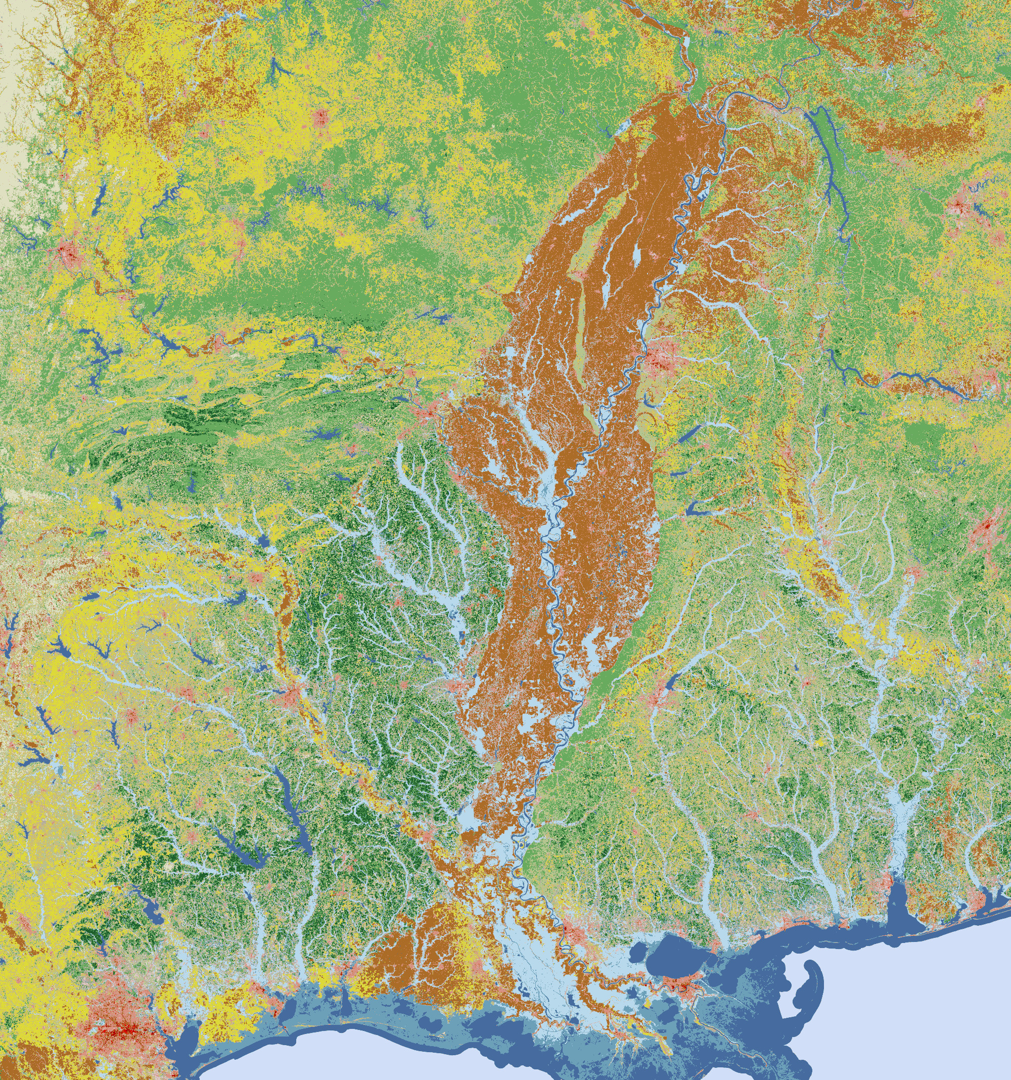
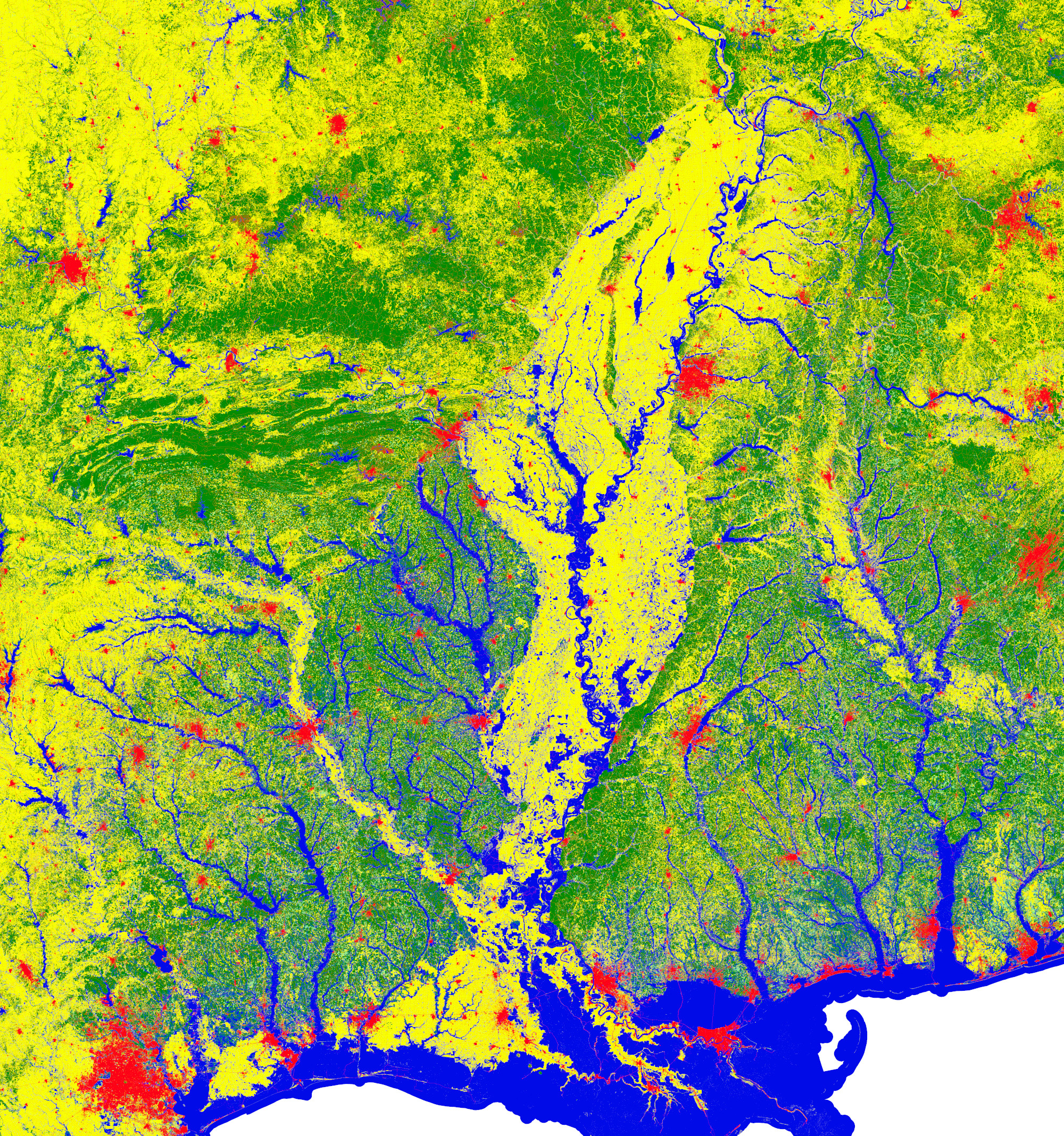
Figure 1. The effect of reclassification: left image – the original land cover(16 classes), right image – the land cover after reclassification (6 classes).
Example 6: area calculation and assigning
The frequently used procedure in raster analysis is a calculation area of patches. Such areas are later assigning to the cells belonging to patches. The resultant layer contains values of patches areas. The described process consists of two steps: calculating areas, and assigning values. It can be done in two calls of plmapcalc. If user decides to use multiple scan of the data file the process can be done in one plmapcalc call.
Assuming that patches are numbered by integers and similarly to calculation of statistics, area calculation needs the vaery simple macro:
  plmapcalc -i patches.tif
            -m 2000
            -e ‘MEM[(int)IN[0]]+=1.0;’
            -s areas.txt
A user has to declare the number of memory cells that is enough to store areas of all patches.
The -m option is followed by maximum patch ID incremented by one.
The next step is to do a reclassification to assign areas’ value to each cell. This step is similar to layer reclassification from example 5 but this time a user has ready to use reclassification file. The macro is as follows:
  plmapcalc -i patches.tif
            -r areas.txt
            -m 2000
            -o areas.tif:Float64:-9999:LZW
            -e ‘OUT[0]=MEM[(int)IN[0]];’
PlMapcalc uses patches.tif file as input once again. During the run, an output file (areas.tif) is created. Cells of this raster file contain areas of patches. The areas are expressed in cells numbers. If it is necessary, a user can scale areas by multiplying cells number by area of a cell.
The result of area calculation for forest districts in Poland is illustrated on figure 2.
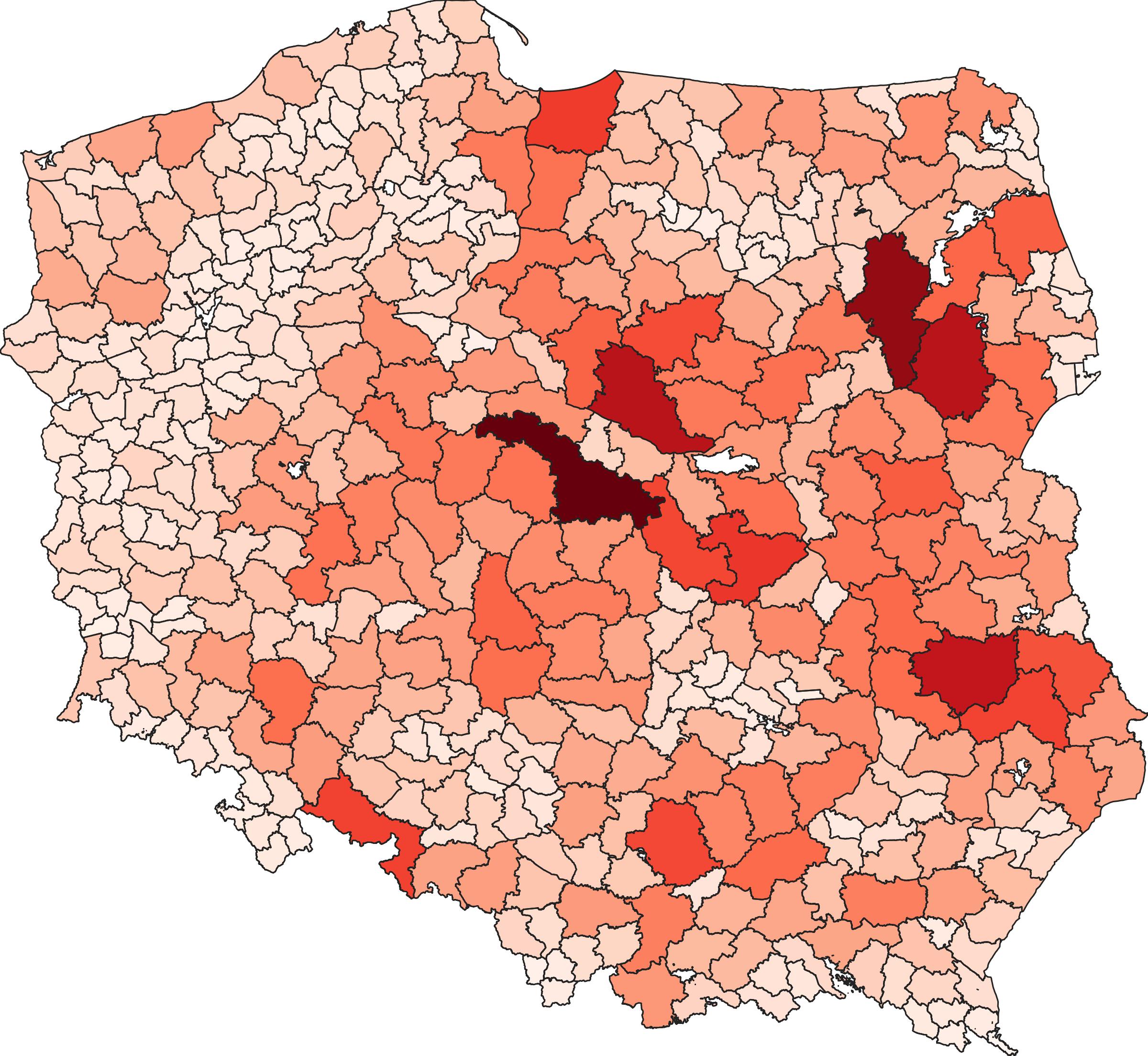
Figure 2. The result of area calculation. The area size is marked with color (white – smallest forest districts, dark red – biggest forest districts).
As it was mentioned at the beginning, it is possible to combine both steps in one run. It can be done with following macro:
  plmapcalc -i patches.tif
            -m 2000
            -o areas.tif:Float64:-9999:LZW
            -e ‘if(ITERATION()==1) MEM[(int)IN[0]]+=1.0;
                else OUT[0]=MEM[(int)IN[0]];’
            --execute-end=‘if(ITERATION()==1) RESTART();’
The results will be exactly the same.
Example 7: space partitioning
PlMapcalc is convenient tool for creating patches with given topology. To create squares that building a rook topology following command is necessary:
  plmapcalc -i reference.tif
            -o sq_patches.tif:UInt32:0:DEFLATE
            -e ‘int size=100;
                OUT[0] = 1 + COL/size + (ROW/size)*(1 + COLS/size);'
The size parameter is for defining size of squares. The reference.tif file provides information about geometry i.e. bounding box, resolution, and the number of rows and columns. The resultant layer will contain patches with the shape of squares. Cells belonging to each patch will contain ID of this patch. Each patch will have unique and greater then zero ID. Value zero is used as no-data marker.
The results of above command run is presented on Figure 3.
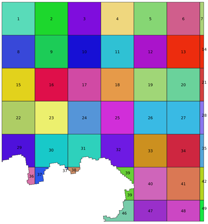
Figure 3. The effect of creating patches with rook topology. Patches are filled with random colors. The labels present IDs of patches.
The rook topology is not only topology that can be created by plMapcalc. The other useful topology is hexagonal grid. To create hexagonal patches a more complicated macro is necessary. The output of the program is similar to former results but this time the patches will have hexagonal shape.
The macro for calculating hexagonal patches (stored in file hexagon.mc):
  int sizeX = 100;
  int size2 = sizeX/2;
  int sizeY = floor(sqrt(3.0)*sizeX/2.0);

  COL++;
  ROW++;

  int R = ROW/sizeY;
  int C = COL/sizeX;

  int Cols = COLS/sizeX + 1;

  int R_center = R*sizeY + size2;
  int C_center = C*sizeX;

  int c,r;
  double d,dx,dy, min_d = 2*sizeX*sizeX;

  for(r=-1; r<2; r++) {
    int Cc = C_center + ((R+r) % 2)*size2;
    int Rc = R_center + r*sizeY;
    if(Cc<0 || Cc>=COLS || Rc<0 || Rc>=ROWS) continue;
    dy = Rc - ROW;
    for(c=-1; c<2; c++) {
      dx = Cc + c*sizeX - COL;
      d = dx*dx + dy*dy;
      if(d<min_d) {
        min_d = d;
        OUT[0] = 1 + C+c + (R+r)*Cols;
      }
    }
  }
The variable sizeX contains size of hexagon’s side. The command to run this macro is following:
  plmapcalc -i reference.tif
            -o hexagons.tif:UInt32:0:DEFLATE2
            -p hexagon.mc
The results of hexagon.mc macro are shown on Figure 4.
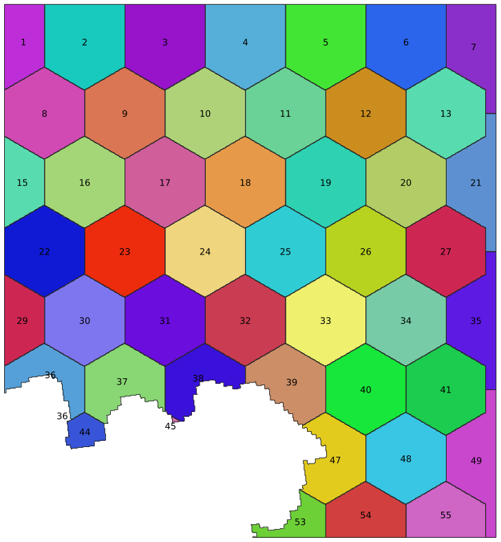
Figure 4. The effect of creating patches with hexagonal topology. Patches are filled with random colors. The labels present IDs of patches.
Example 8: Thiessen (Dirichlet/Voronoi) tessellation
Thiessen tessellation can be created with plMapcalc. To do that it is needed to create memory file containing points coordinates. Let’s create following file and save it as xy_coordinates.txt:
     0 4749361.26105342
     1 3114579.6505474
     2 4759413.25837782
     3 3123209.19542023
     4 4764059.93638626
     5 3098648.18308986
     6 4751068.2039953
     7 3097036.07031142
     8 4778568.95139223
     9 3111924.40597114
    10 4789948.57100476
    11 3096182.59884048
    12 4781129.36580505
    13 3066121.43703073
    14 4793077.9663982
    15 3073518.18977887
    16 4776862.00845036
    17 3088596.18576547
    18 4790991.70280257
    19 3121976.40329554
Even memory cells contain X coordinate of sampled points, and odd memory cells contain Y coordinate. Then, one can run plMapcalc with BEGIN and CELL macros:
  plmapcalc -i reference.tif
            -o thiessen.tif:UInt32:0:DEFLATE2
            -r xy_coordinates.txt
            --execute-begin=’int i, r, c;
                             double x, y;

                             for(i=0; i<MEMNUM; i=i+2) {
                               x = MEM[i];
                               y = MEM[i+1];
                               c = (x - GEOTRANS[0])/GEOTRANS[1];
                               r = (y - GEOTRANS[3])/GEOTRANS[5];
                               MEM[i] = c;
                               MEM[i+1] = r;
                             }‘
            --execute=’double dx, dy, d, min_d = 2*ROWS*COLS;
                       int i;

                       OUT[0] = 0.0;

          		       for(i=0; i<MEMNUM; i=i+2) {
          			     dy = MEM[i+1] - ROW;
          			     dx = MEM[i] - COL;
          			     d = dx*dx + dy*dy;

          			     if(d<min_d) {
          			       min_d = d;
          			       OUT[0]=1+i/2;
          			     }
          		       }‘
The BEGIN macro takes (x, y) coordinates as input and converts them to (col, row) coordinates.
The CELL macro finds a closest point and assigns its order number to the current point. The resultant output layer is shown on Figure 5.
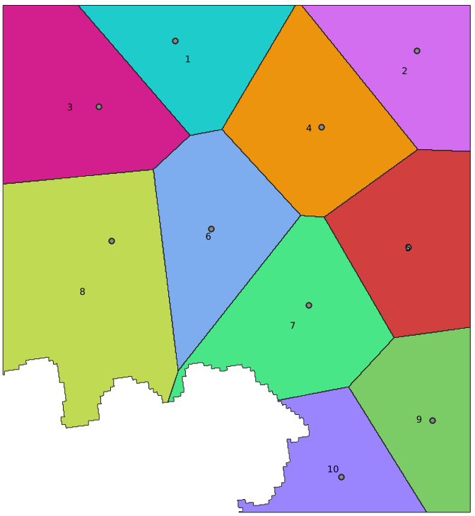
Figure 5. The effect of Thiessen tessellation. Thiessen polygons are filled with random colors. The labels present IDs of the polygons. The seeds are marked by gray points.
Example 9: image histogram matching and equalization
This is an implementation of the algorithm to equalize greyscale image histogram. It is a special case of histograms matching. The main aim of histogram matching is to make two histograms similar each other. In histogram equalization, reference histogram is linear.
Figure 6 shows the original image (on the left) and the image after applying histogram equalization (on the right). The result is made by plMapcalc script.

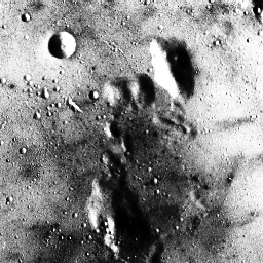
Figure 6. The effect of histogram equalization. The left image histogram is equalized to stretch the contrast and make details visible.
This example shows how to use two input data scans. During first scan, lookup table is bulit. In the second scan, the lookup table is used to reclassify input image. ITERATION function allows to control processing flow. RESTART function is used to jump at the beginning of the data.
This plMapcalc call will do histogram equalization:
  plmapcalc --input=greyscale_input.tif
            --memory=1000
            --output=grey_eq_output.tif:Int32
            --execute-begin='int i;

                             // creating reference CDF
                             for(i=0; i<256; i++)
                               MEM[i] = i/256.0;'
      		--execute='if(ITERATION()==1)
                         // building image histogram
                         MEM[(int)IN[0]+500]+=1;
                       else
                         // reclassyfication of the input
                       OUT[0]=MEM[(int)IN[0]+500];'
      		--execute-end='if(ITERATION()==1) {
                             int i, j, min_j;
                             double v, a, min_v;

                             // calculating image CDF
                             for(i=1+500; i<256+500; i++)
                               MEM[i]+=MEM[i-1];
                             v=MEM[255+500];
                             for(i=500; i<256+500; i++)
                               MEM[i]/=v;

                             // reclassification rules
                             for(i=500; i<256+500; i++) {
                               v=MEM[i];
                               min_j=0;
                               min_v=fabs(MEM[0]-v);
                               for(j=1; j<256; j++) {
                                 a=fabs(MEM[j]-v);
                                 if(a<min_v) {
                                   min_j=j;
                                   min_v=a;
                                 }
                               }
                               MEM[i]=min_j;
                             }
                             RESTART();
                           }'
Histogram matching is very similar to histogram equalization. The only difference is the reference histogram is not artificial (linear) but it is built from reference image. The results of histogram matching are presented on figure 7.
This plMapcalc call will do histogram matching:
  plmapcalc --input=greyscale_input.tif
            --input=greyscale_reference.tif
            --memory=1000
            --output=grey_eq_output.tif:Int32
            --execute-begin='int i;
                             // creating reference CDF
                             for(i=0; i<256; i++)
                               MEM[i] = i/256.0;'
            --execute='if(ITERATION()==1) {
                         // building image histograms
                         MEM[(int)IN[0]+500]+=1;
                         MEM[(int)IN[1]]+=1;
                       } else
                         // reclassyfication of the input
                         OUT[0]=MEM[(int)IN[0]+500];'
            --execute-end='if(ITERATION()==1) {
                             int i, j, min_j;
                             double v, v_in, v_ref, a, min_v;

                             // calculating image CDFs
                             for(i=1; i<256; i++) {
                               MEM[i+500]+=MEM[i-1+500];
                               MEM[i]+=MEM[i-1];
                             }
                             v_in=MEM[255+500];
                             v_ref=MEM[255];
                             for(i=0; i<256; i++) {
                               MEM[i+500]/=v_in;
                               MEM[i]/=v_ref;
                             }

                             // reclassification rules
                             for(i=500; i<256+500; i++) {
                               v=MEM[i];
                               min_j=0;
                               min_v=fabs(MEM[0]-v);
                               for(j=1; j<256; j++) {
                                 a=fabs(MEM[j]-v);
                                 if(a<min_v) {
                                   min_j=j;
                                   min_v=a;
                                 }
                               }
                               MEM[i]=min_j;
                             }
                             RESTART();
                           }'
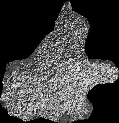

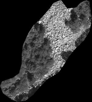
Figure 7. The effect of histogram matching. The reference image is on the left. The middle image histogram is matched to obtain an image that can be processed in further analysis together with the reference.
Example 10: Laplace operator calculation for an image
The Laplace operator can be used to analyze the image for edge detection. In the discrete version and considering 8 directions, the Laplace operator can be written as:
             -1  -1  -1
             -1   8  -1
             -1  -1  -1
plMapcalc allows you to calculate the Laplace operator using layer shifting. The offset is defined by specifying additional parameters when defining the input layer. The syntax looks as follows:
-i layer_name.tif:band_no:shift_x:shift_y
where shift_x and shift_y are the number of raster cells by which the layer is shifted in the horizontal and vertical axis, respectively. A negative value of shif_x means that the program takes into account the cells to the left of the central cell. Correspondingly, for the vertical axis, a negative shift_y value means cells above the central cell.
The full syntax of the plMapcalc command (calculation uses eight directions, the band number is skipped, by default the first band is taken for calculations):
    plmapcalc -i input.tif -i input.tif::-1:-1 -i input.tif::-1:0 -i input.tif::-1:1
              -i input.tif::0:-1 -i input.tif::0:1 -i input.tif::1:-1 -i input.tif::1:0
              -i input.tif::1:1
              -o output.tif:Byte
              -e 'int i; OUT[0]=8*IN[0]; for(i=1; i<9; i++) OUT[0]-=IN[i];'
The source image, the grayscale photo, and the result of the program are illustrated in Figure 8.
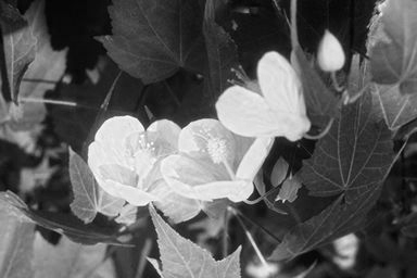
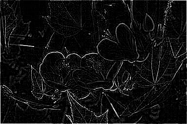
Figure 8. On the left, the source image in grayscale. On the right, the result of the calculation.
Example 11: implementation of Koeppen-Geiger climate classification
Koeppen-Geiger climate classification needs information about temperature and precipitation. This information should be collected for each month of the year. Such data can be downloaded from WoldClim project (http://www.worldclim.org).
Let’s assume that the user has downloaded all necessary layers and stored them as:
- temperature layers: t01.tif, t02.tif, …., t12.tif
- precipitation layers: p01.tif, p02.tif, …., p12.tif
Each temperature layer contains information about multiyear average of monthly temperature. Each precipitation layer contains information about multiyear average of monthly sum of precipitation.
Spinoni provided convenient algorithm to do KG classification. In the example, classification to 13 climate classes is presented (Spinoni et al. (2015): Towards identifying areas at climatological risk of desertification using the Köppen–Geiger classification and FAO aridity index, Int. J. Climatol. 35: 2210–2222). Rules to classify climate data are too complex to insert as a command line parameter. For such a case, plMapcalc has an ability to read macro from a file.
Contents of the macro file (KG_classification_13.mc) is shown below:
  // KG classes
  #define EF  1
  #define ET  2
  #define BW  3
  #define BS  4
  #define Am  5
  #define Aw  6
  #define Af  7
  #define CS  8
  #define CW  9
  #define CF 10
  #define DS 11
  #define DW 12
  #define DF 13

  // Temperature 10*C deg.

  double Tcold  =  10000.0;
  double Thot   = -10000.0;
  double Tmon10 =  0.0;
  double Ta;
  double MAT  = 0.0;
  double MATw = 0.0;
  double MATs = 0.0;
  int i;

  for(i=1; i<=12; i++) {
    Ta = IN[i-1];
    if(Ta<Tcold) Tcold=Ta;
    if(Ta>Thot) Thot=Ta;
    if(Ta>100.0) Tmon10+=1.0;
    MAT+=Ta;
    if((i>3) && (i<10)) {
      // summer
      MATs+=Ta;
    } else {
      // winter
      MATw+=Ta;
    }
  }
  Tcold  *= 0.1;
  Thot   *= 0.1;
  Tmon10 *= 0.1;
  MAT    /= 120.0;

  // Precipitation mm/month

  double MAP  = 0.0;
  double MAPw = 0.0;
  double MAPs = 0.0;
  double Pr;
  double Pdry  = 10000.0;
  double Pwdry = 10000.0;
  double Psdry = 10000.0;
  double Pwwet = 0.0;
  double Pswet = 0.0;

  for(i=1; i<=12; i++) {
    Pr=IN[i-1+12];
    if(Pdry>Pr) Pdry = Pr;
    MAP += Pr;
    if((i>3) && (i<10)) {
      // summer
      if(Psdry>Pr) Psdry = Pr;
      if(Pswet<Pr) Pswet = Pr;
      MAPs+=Pr;
    } else {
      // winter
      if(Pwdry>Pr) Pwdry=Pr;
      if(Pwwet<Pr) Pwwet=Pr;
      MAPw+=Pr;
    }
  }

  double p;
  double Pthre;

  // Summer/winter
  if(MATw > MATs) {
    p=MAPw; MAPw=MAPs; MAPs=p;
    p=Pwdry; Pwdry=Psdry; Psdry=p;
    p=Pwwet; Pwwet=Pswet; Pswet=p;
  }

  // P threshold
  if(MAPw > 0.7*MAP)
    Pthre= 20.0*MAT;
  else if(MAPs > 0.7*MAP)
    Pthre = 20.0*MAT+280.0;
  else
    Pthre = 20.0*MAT+140.0;

  int alpha, beta, delta;

  alpha=((Psdry<30.0) && (Psdry<Pwwet/3.0) && (MAPs<MAPw));
  beta=((Pwdry<Pswet/10.0) && (MAPw<MAPs));
  delta=!(alpha && beta);

  int KG=0;

  if(Thot<10.0) {
    if(Thot>0.0)
      KG=ET;
    else
      KG=EF;
  } else {
    if(Pthre>=MAP) {
      if(MAP<Pthre/2.0)
        KG=BW;
      else
        KG=BS;
    } else {
      if(Tcold>=18.0) {
        if(Pdry<60.0) {
          if(Pdry>=100.0-MAP/25.0)
            KG=Am;
          else
            KG=Aw;
        } else
          KG=Af;
      } else if(Tcold<-3.0) {
        if(alpha)
          KG=DS;
        else if(beta)
          KG=DW;
        else if(delta)
          KG=DF;
      } else {
        if(alpha)
          KG=CS;
        else if(beta)
          KG=CW;
        else if(delta)
          KG=CF;
      }
    }
  }

  OUT[0] = (double)KG;
The macro contains many different C syntax elements such as
- constants definitions,
- local variables definition and initialization,
- logical, integer, and double variables,
- conditional expressions,
- type casting and conversion,
- comments.
Command line call of mapcalc should be following:
  plmapcalc -i t01.tif -i t02.tif -i t03.tif -i t04.tif -i t05.tif
            -i t06.tif -i t07.tif -i t08.tif -i t09.tif -i t10.tif
            -i t11.tif -i t12.tif
            -i p01.tif -i p02.tif -i p03.tif -i p04.tif -i p05.tif
            -i p06.tif -i p07.tif -i p08.tif -i p09.tif -i p10.tif
            -i p11.tif -i p12.tif
            -o kg13.tif:Byte:0:LZW
            -p macros/KG_classification_13.mc
plMapcalc will read data from 24 input files and create one output file. The resultant file will be type of Byte where no-data cells will contain value zero. The value zero will be defined as no-data value. This file will be compressed with LZW algorithm. plMapcalc will read macro from file KG_classification_13.mc placed in subdirectory macros. The file suffix mc is optional. The order of input files is significant.
The results of above script are presented on Figure 9 (Netzel P., Stepinski T.F, 2016: On using a clustering approach for global climate classification. Journal of Climate. Vol. 29, no 9, pp.3387–3401)
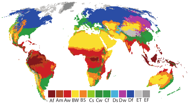
Figure 9. The Koeppen-Geiger climate classification obtained by plMapcalc script.